Home | English articles

GENETICALLY PREFERRED ANCESTRAL LINES IN SEXUAL BEINGS

The splitting proportions in the ascendency in sex-linked inheritance in human beings

By Arndt Richter, Munich, Germany

	Summary On the basis of the regularity of the transmission of the X-Y chromosomes and the ancestral structure of sexual beings, typical splitting proportions can be postulated as inheritance probability values in the ascendance. The derivation is carried out in the example of a normal human genealogical chart. Result: Each position in a genealogical chart is determined by fixed "inheritance probability values" in respect to the sex chromosomes. This results in inherited dominant genealogical lines as well as in areas of the chart in which there can be no question of sex chromosome transmission. There are basic differences between male and female probands in the genealogical chart. The splitting proportions in the individual generations follow the so-called Fibonacci sequence and are thus closely connected with the relationship of the so-called Golden Ratio ( j = 1,618034..), which seems to play a significant role in nature and art. * * * * * * *
	Over six decades have passed since Thomas Hunt Morgan (1866-1945) and his co-worker Calvin B. Bridges (1889-1938) discovered sex-linked inheritance in the fruit fly Drosophilia melanogaster, "the geneticist's pet". In 1916 Morgan was able to announce: "We now know how the factors of heredity carried by the parents are sorted out to the germ cells". Up to the presence, however, there still exists uncertainty as to whether there are genetically predominant lines in a genealogical chart. (see notes 1-7). Today all hypotheses and theories concerning the matter seem to be rejected. (see note 8). A basis for the inherited predominance of certain genealogical lines is given here on the basis of sex-chromosome linked inheritance, called sex-linked for short. As is known, the normal chromosomes (autosomes) follow Mendelian rules independently of each other after the basic split. Therefore there is no basis for the predominance of one or several genetic lines in them. It is different, however, for the sex chromosomes, which are taking a special position. As we know, above all they are carriers of all sex-linked hereditary factors. Although the essentially larger X chromosomes may play the major role in transmission of hereditary factors, the "catalytic", presumably even "directing" role of the Y chromosome surely is not less significant. The significance of the sex chromosomes vis a vis the autosomes scarcely needs further description. It will suffice to indicate their function in determining sex. All primary and secondary sex characteristics and differences must basically be attributed to these chromosomes. The extent of joint action with the autosomes is of lesser significance here in the derivation of basic numerical relationships. Since the chromosome combinations XX or XY alone determine whether the result will be male or female, the significance of these chromosomes prominent (we will ignore the abnormal chromosome aberrations XXX or XYY here). Also significant are the qualitative differences of these chromosomes within the individuals. We will disregard completely further abnormal deviations. The "scope of the normal" offers a wealth of fascinating possibilities regarding individual differences in characters. The transmitting role of the X chromosomes for certain sex-linked diseases (e.g., hemophilia, red-green color blindness, microphthalmia, some tooth diseases) is particularly instructive (indicator!) for the tracing of the inheritance line and thereby also of great interest for biological genealogy; furthermore the topic still has great practical medical importance (see extensive literature). Yet all of this can be disregarded for the following considerations of probability, as well as the fact of chromosome mutation and crossing-over. Moreover, genes in the differential segment of the sex chromosomes never show crossing over; they always remain in the same chromosome, and are carriers of strictly sex-linked inheritance (see note 9). The X-Y mechanism is obviously valid for all sexual creatures, sometimes with certain deviations (bees). In birds and some insects, the male sex is characterized (XX), while in fish and apparently all mammals this is the female sex. The inheritance of the sex chromosomes in the human being is, as we know, designated as follows: The father transmits his X chromosome, which he received exclusively from his mother, only to his daughters. The second X chromosome, which is determining for the female sex, is received by daughters only from the mother, who always transmits fortuitously one of her two X chromosomes to her male or female children. The sons receive their only X chromosome exclusively from the mother, while the Y chromosome that determines the male sex is transmitted exclusively by the father. This will result in different inheritance probabilities for the individual relationship lines. 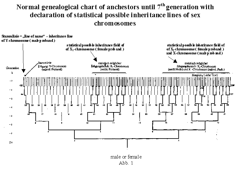This will be explained by the example of a human genealogical table. Like every genealogical table of a sexual creature, that of the human shows a strictly regular structure. The descendants' chart, on the other hand, shows an irregular structure due to the varying numbers of children. The regular composition of the ascendants' chart is because each individual has no more and no fewer than 2 parents; that is probably the only irrefutable law of genealogy. Thus, the number of ancestors in each generation k is unambiguous, namely equal to the k-power of 2 (2k). The ancestor numbers in Table 1 follow the usual nomenclature of today according to Kekule, but are otherwise without significance for the relationships derived here; every other clear designation on the genealogical chart leads to the same result. The proband (= person under investigation, male or female) has the number 1, the father 2, the mother 3, etc. (Table 1). The father of ancestor n always has the number 2n, the mother 2n + 1. All male persons (except the proband himself) carry even numbers, all female persons uneven numbers. Every generation begins with the numerical value of the appropriate power of 2 as the ancestor number. This line is the principal line, also called the purely male line or the name line. In Table 1 the child is always designated by a vertical line down from the middle of the two parents. So much for the structure and labeling of the genealogical chart. A male person, for example the proband number 1 himself, receives his X chromosome with certainty (probability 1) from his mother (number 3) only. She herself, however, inherited this chromosome either from her father (number 6) or from her mother (number7), and with equal probability, so that both probability values are halved in the transmission to the next generation (see table 2). Therefore the probability is 0.5 for each. From ancestor number 6 the probability value does not chance in the transmission to the next generation, since ancestor number 6, as a male. can receive his X chromosome only from his mother (number 13); the probability of number 13 therefore remains 0.5. While for the female ancestor number 7, parents number 14 and number 15 come into play as transmitters with equal probability, the probability values therefore are halved again in the transmission to the next ancestral generation (probability of number 14 and number 15 is 0.25 each). This will suffice as a description of disproportionization. The Y chromosome, always passed only from father to son, has a completely unambiguous inheritance line on the genealogical chart. The probability value for the Y chromosome within the principal line is therefore always 1, independent of the generation. If, for example, in the case of a great-grandson, the entire legacy has disappeared in the individual case, his Y chromosome still remains fully preserved. In table 2, the probability values are given for all ancestors up to the generation k = -6. The nomenclature is that of today's scholarly genealogy. Naturally the b values in the chart for the X chromosome (bx for the man, bx1 and bx2 for the woman) are always 0 or 1 [because of crossing over, 0 or 1 is valid stritcly speaking only for single genes, which are localized on the X chromosome!] in the individual case, namely 1 only once in each ancestral generation (in the case of one ancestor) and 0 in all other positions (note 10). Those positions on the genealogical chart marked with a line in table 2 are eliminated for an inheritance probability of the sex chromosomes on the basis of the X-Y mechanism. There are "free places" and "new" areas in each higher ancestral generation. The percentage of "free places" becomes increasingly bigger within the chart as one goes back in time. The "free places" can in given cases be filled in the case of multiple inheritance (for example, ancestor 12, if the same as ancestor 10, (if ancestor 6 and 7 are brother and sister) female proband; see illustration 3c). Such ancestral charts, which show loss of ancestors, also called ancestral implex, will, however, not be looked at more closely in these basic considerations within the first ancestral generations. Admittedly, loss of ancestors will be the rule in higher generations, and the "pure" numerical relationships will be obscured, partially through "shifting of generations", such as niece-uncle marriages. In our civilization, marriages of close relatives are no rarities. 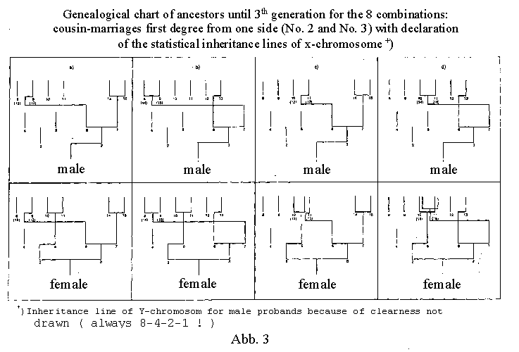The eight different possible combinations of a cousin-aunt marriage of the first degree on one side are shown in figure 3 a-d and figure 4 (here there are only six rather than eight different great-grandparents!). Figure 4 gives all inheritance probability values for these eight combinations, limited to the third generation, k = -3. All possible inheritance lines for the sex chromosomes for seven generations can be seen clearly in figure 1. It is differentiated between male and female probands. For the individual inheritance case of the X chromosomes designated x1 and x2 it is a question of only one single line. For example, for x2 , such a line is 238-119-59-29-14-7-3-1. Moreover, from the seventh generation on, there are twenty additional inheritance lines, some with greater, some with lesser statistical probability. From the two illustrations it is clear that there are basic differences between ancestral charts with male and female probands. The author is not aware that this fact has been referred to previously in the scientific literature. The genealogical table of a male proband is characterized on the one hand by the clear transmission of the Y chromosome within the so-called male line, and on the other hand by the inheritance probability field of the single X chromosome. The genealogical table of a female proband is characterized by two independent inheritance probability fields for the two X chromosomes (X1 and X2). Thus the X2 field of a female proband is identical with the X field of a male proband. The possible inheritance paths for the eight combinations of cousin marriages to the third generation can be seen in illustration 3, where only the transmission of the X chromosomes is shown. From the bx -values (mean biological relationship share) of the chart, one can derive the "splitting proportions" p, which, for example, assume the following forms in the case of bx2 - values ranked by size: k = p = sk = -1 1 1 -2 1:1 2 -3 2:1:1 3 -4 2:2:2:1:1 5 -5 4:2:2:2:2:2:1:1 8 -6 4:4:4:4:2:2:2:2:2:2:2:1:1 13 -7 8:4:4:4:4:4:4:4:4:4:2:2:2:2:2:2:2:2:2:1:1 21 sk is the number of bx -values in each generation. Presumably these proportions were overlooked previously because of the predominating way of observing descendants. The biometric and biostatistics structure of the Mendelian laws is after all mostly directed toward the future-oriented question "where to?". The question "from where" is less modern, but nevertheless of equal scientific interest. Now we come upon an interesting mathematical number series that comes to light in the probability values: namely that the numbers s of the bx -values within the individual ancestral generations follow the so-called Fibonacci number sequence 1,1,2,3,5,8,13,21,34,….. Each member results from the sum of the two preceding ones: an+2 = an + an+1 The bx inheritance probability values between the female and male ancestors in each generation also demonstrate the relationship of the Fibonacci numbers, e.g., in the seventh ancestral generation: 13 female and 8 male. Geppert (see note 11) indicates the following relation to for the Fibonacci sequence by induction: , where w represents the "golden ratio" relationship 0.618034… Further: and In Geppert's work w appears in the descendancy in processes of selection and incest. To the best of my knowledge, it was Rösch (see note 12) who first referred to the Fibonacci numbers in the ascendency, namely in an extreme case of an incestual ancestral chart showing continuous child-parent marriages. The theoretical number of ancestors increases in the individual ancestral generations according to this sequence. Further on, Rösch discovered the Fibonacci number sequence obviously as a physical number of ancestors in the ancestral chart of bees (see note 13). This chart, however, is in an exceptional situation because of its peculiar regularity, since each male bee descends only from a female bee, while each female bee derives from a pair of parents. In the inheritance line of the X chromosomes, however, this number sequence is on another level. In the normal ancestral chart of all sexual beeings reproducing in the usual way, it is the probability number sequence according to the generation. Actually, the following ist not part of the main topic we discuss here. This was in appreciation of the 80th birthday of Prof. Dr. Siegried Rösch, Wetzlar. Rösch (see note 14) sees in the number j (the reciprocal value of w), the only positive number whose reciprocal value results from subtraction from 1 as now shown: , a "world constant": "Our number j has shown such a many-sided significance that it appears worthy of being regarded as a 'world constant', like the Ludolf number p  = 3.141592… or the basis of natural logarithms, e = 2.718281.... (both are likewise infinitely long decimal numbers without recurring decimal)." In examples from inanimate and animate nature as well as in works of art, Rösch clearly refers to the Fibonacci numbers and the Golden Ratio relationship. Johannes Keppler called the recognition of this "divine division" a "precious jewel"! We cannot pursue here the further theoretical structure of the X / Y - chromosome transmission in cases of multiple relationship. We cannot even touch upon the practical significance for the breeding of animals, and even plants, of the relationships presented here. All this, as well as possible consequences for the knowledge theory, will have to be followed by those who are more qualified. In Volume 75 we will treat briefly the connections of these findings with descendancy. The original essay Erbmäßig bevorzugte Nachfahrenlinien durch geschlechtsgebundene Vererbung is published here for the first time. An english translation is soon to be released.
	Remarks / Sources: Arthur Schopenhauer: Die Welt als Wille und Vorstellung. Bd. 2, 43. Kapitel (Erblichkeit der Eigenschaften), Leipzig 1844. Robert Sommer: Bericht über den II. Kurs mit Kongreß für Familienforschung, Vererbungs- und Regenerationslehre in Gießen vom 9.-13. 4. 1912, Halle a. S. (Marhold) 1912, S. 13 f. Hammer : Med. Klinik 1912, Nr. 25, und in o. g. "Kursbericht"; 2, S. 82. Wilhelm Karl Prinz v. Isenburg: Über Ahnentafelforschung. Leipzig (Degener) 1926, S. 10 f, S. 15 f u. S. 21 f. Otto Forst de Battaglia: Wissenschaftliche Genealogie. Bern 1948 (= Sammlung Dalp, Bd. 57), S. 35 f. u. S. 162 ff. Felix v. Schroeder: Mitteilungen der Zentralstelle für Deutsche Personen- und Familiengeschichte, Leipzig 1936, H. 57: Ahnentafeln, Stammtafeln und Nachfahrentafeln (II. Erbkunde), S. 11 f. Theodor Aign: Zum Problem der Nachkommen- und Ahnengleichheit. Analyse der Nachkommentafeln Karls d. Gr. und der Ahnentafeln verschiedener Hersbrucker Probanden. In: Reichsstadt Nürnberg, Altdorf und Hersbruck. Bd. 6 der Freien Schriftenfolge der Gesellschaft für Familienforschung in Franken. Nürnberg 1954, S. 79. Heinz F. Friederichs: Handbuch der Genealogie von E. Henning und W. Ribbe, Neustadt a. Aisch (Degener) 1972, Kapitel Humangenetik, S. 233. Hedi Fritz-Niggli: Vererbung bei Mensch und Tier. Stuttgart (Thieme) 1961, S. 71. Hermann v. Schelling: Das Alles- oder Nichts-Gesetz, gedeutet als Endergebnis einer Auslösungsfolge. Abh. preuß. Akad. Wiss. (1944) math.-nat. Kl., N. 6, 25 S. Harald Geppert und Siegfried Koller: Erbmathematik. Theorie der Vererbung in Bevölkerung und Sippe. Leipzig (Quelle und Meyer) 1938, S. 82 und S. 115 f. Siegfried Rösch: Grundzüge einer quantitativen Genealogie. Heft 31 des Praktikums für Familienforscher. Neustadt a. Aisch (Degener) 1955, S. 26 u. Fig. 17; auch erschienen als Teil A des Buches : Goethes Verwandtschaft. Versuch einer Gesamtverwandtschaftstafel mit Gedanken zu deren Theorie. Neustadt a. Aisch (Degener) 1956, S. 26, Fig. 17. Siegfried Rösch: Die Ahnenschaft einer Biene. Genealogisches Jahrbuch 6/7 (1967), S. 5-11, und Kongreßbericht "Genealogica et Heraldica" 1, Wien (1970), S. 131-133. Siegfried Rösch: Mathematik in Spiralen oder der überraschungsreiche "Goldene Schnitt". Neues Universum (Stuttgart) 94 (1977) S. 301-310.

Fig. 1

Fig. 2 (Table 2):

Fig. 3:

Fig.4 /Table 4

top